Unsupervised clustering with general GMCMs
Source:vignettes/usage-example-general-model.Rmd
usage-example-general-model.RmdThis is a quick tutorial for using the general GMCM for unsupervised clustering.
Initialization
The GMCM1 package is loaded.
If GMCM is not installed, please uncomment the above line and rerun the script to install from CRAN. The development version can be installed from GitHub following the instructions there.
Simulation of data
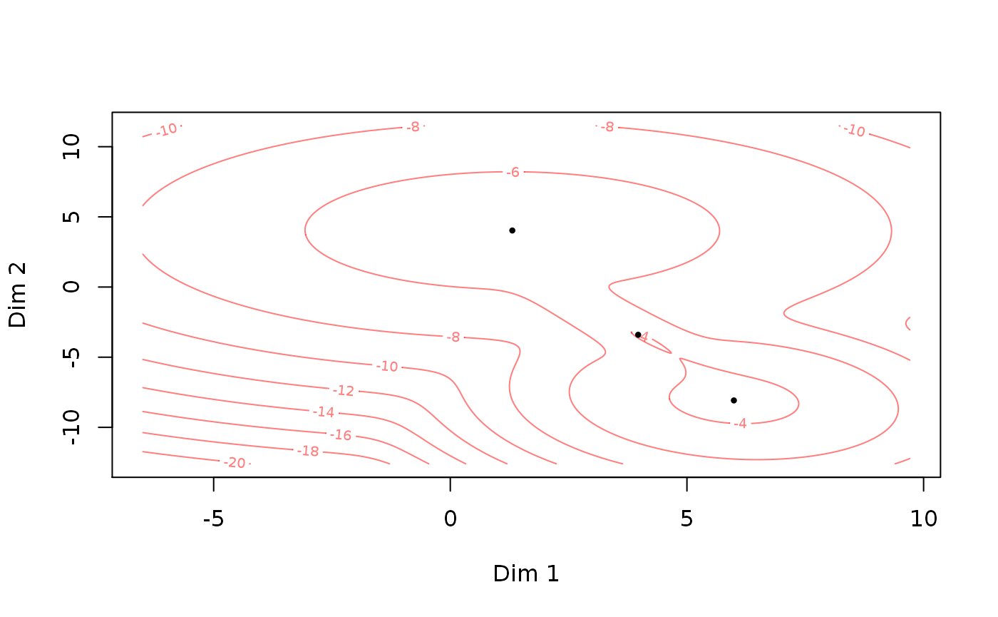
First, we simulate some toy data. We wish to simulate, say, 1000 observations of 2-dimensions each of which stems from one of 3 components. In order to do so, we construct a parameter object theta and simulate from the GMCM.

ds <- SimulateGMCMData(n = 1000, theta = true_theta)
str(ds)
## List of 4
##  $ u    : num [1:1000, 1:2] 0.0452 0.5879 0.8876 0.0706 0.4786 ...
##  $ z    : num [1:1000, 1:2] -2.71 5.19 7.37 -1.77 4.46 ...
##  $ K    : int [1:1000] 3 3 1 3 1 1 3 1 1 1 ...
##  $ theta:List of 5
##   ..$ m    : num 3
##   ..$ d    : num 2
##   ..$ pie  : Named num [1:3] 0.5084 0.0989 0.3928
##   .. ..- attr(*, "names")= chr [1:3] "pie1" "pie2" "pie3"
##   ..$ mu   :List of 3
##   .. ..$ comp1: num [1:2] 5.99 -8.08
##   .. ..$ comp2: num [1:2] 3.97 -3.4
##   .. ..$ comp3: num [1:2] 1.31 4.03
##   ..$ sigma:List of 3
##   .. ..$ comp1: num [1:2, 1:2] 2.55 -0.44 -0.44 3.77
##   .. ..$ comp2: num [1:2, 1:2] 1.06 -1.6 -1.6 3.19
##   .. ..$ comp3: num [1:2, 1:2] 11.2561 -0.0595 -0.0595 10.2816
##   ..- attr(*, "class")= chr "theta"
As can be seen, the SimulateGMCMData function returns a list containing the copula observations u, the unobserved process z, the latent groups K, and the theta used for simulation.
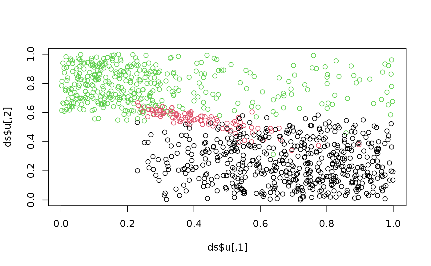
Plotting the true copula realizations and coloring by the true classes shows what we intend to estimate and recover:
plot(ds$u, col = ds$K)

A ranking of u (or z) corresponds to what would be the data in a real application.

Initial parameters
To fit a general GMCM, we must choose some initial parameters. The choose.theta is a (sometimes) helpful default we here invoke explicitly:
init_theta <- choose.theta(uhat, m = 3)
print(init_theta)
## theta object with d = 2 dimensions and m = 3 components:
##
## $pie
##  pie1  pie2  pie3
## 0.300 0.345 0.355
##
## $mu
## $mu$comp1
## [1] 0 0
##
## $mu$comp2
## [1] -2.097679  1.557202
##
## $mu$comp3
## [1]  1.039218 -1.846066
##
##
## $sigma
## $sigma$comp1
##      [,1] [,2]
## [1,]    1    0
## [2,]    0    1
##
## $sigma$comp2
##           [,1]     [,2]
## [1,] 0.4001925 0.000000
## [2,] 0.0000000 0.489384
##
## $sigma$comp3
##           [,1]      [,2]
## [1,] 0.8003757 0.0000000
## [2,] 0.0000000 0.5226159
The function needs to know how many components we want to estimate though this number may very well be unknown in practice.
Model fitting
With the data loaded and defined initial parameters, the model is now fitted.
est_theta <- fit.full.GMCM(u = uhat,  # Ranking function is applied automatically
                           theta = init_theta,
                           method = "NM",
                           max.ite = 5000,
                           verbose = FALSE)
print(est_theta)
## theta object with d = 2 dimensions and m = 3 components:
##
## $pie
##      pie1      pie2      pie3
## 0.2085000 0.2745018 0.5169982
##
## $mu
## $mu$comp1
## [1] 0 0
##
## $mu$comp2
## [1] -3.1515792  0.8279297
##
## $mu$comp3
## [1]  0.8631953 -1.5608324
##
##
## $sigma
## $sigma$comp1
##           [,1]      [,2]
## [1,] 1.0000000 0.3978458
## [2,] 0.3978458 1.0000000
##
## $sigma$comp2
##             [,1]        [,2]
## [1,]  1.49969539 -0.01741992
## [2,] -0.01741992  0.43467752
##
## $sigma$comp3
##            [,1]       [,2]
## [1,]  0.2798609 -0.0292142
## [2,] -0.0292142  0.1083622
The fitting method is set to "NM" with a maximum number of iterations of 100.
Unsupervised clustering
The estimated parameters are used to calculated posterior component probabilities on which the classification is based:
## int [1:1000] 2 1 3 2 3 3 2 3 3 1 ...If it is of interest, the posterior probability can be computed directly using
post_prob <- get.prob(uhat, est_theta) # Compute component probabilities
Results
The number of observations in each class can be e.g. counted by
table(membership)
## membership
##   1   2   3
## 200 272 528
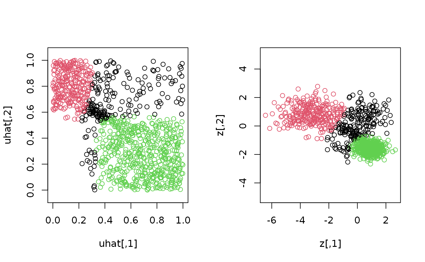
The results are also displayed by plotting
par(mfrow = c(1,2))
plot(uhat, col = membership, asp = 1) # Plot of estimated copula values
z <- GMCM:::qgmm.marginal(uhat, theta = est_theta) # Estimate latent process
plot(z, col = membership, asp = 1) # Plot of estimated latent process

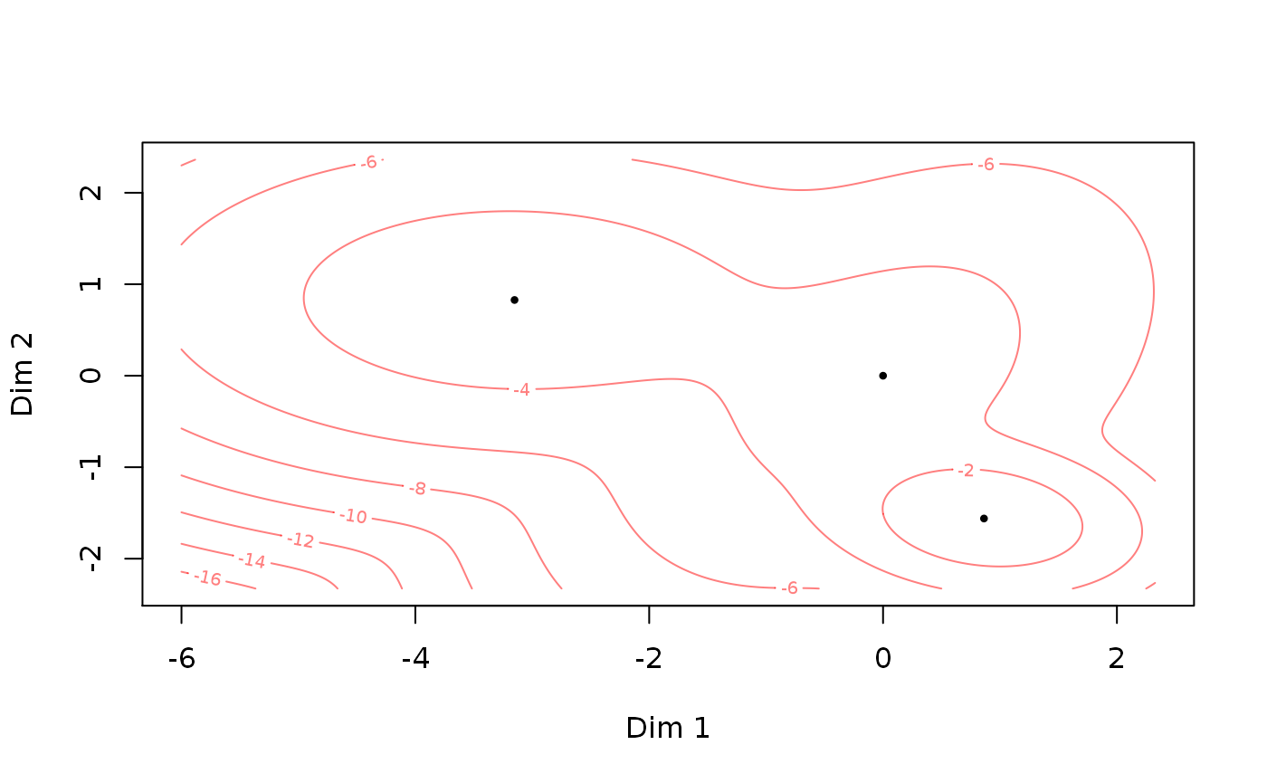
The fitted theta object can also be plotted directly:
plot(est_theta)

Session information
This report was generated using rmarkdown2 and knitr3 under the session given below.
## R version 4.0.2 (2020-06-22)
## Platform: x86_64-pc-linux-gnu (64-bit)
## Running under: Ubuntu 16.04.6 LTS
##
## Matrix products: default
## BLAS:   /usr/lib/openblas-base/libblas.so.3
## LAPACK: /usr/lib/libopenblasp-r0.2.18.so
##
## locale:
##  [1] LC_CTYPE=en_US.UTF-8       LC_NUMERIC=C
##  [3] LC_TIME=en_US.UTF-8        LC_COLLATE=en_US.UTF-8
##  [5] LC_MONETARY=en_US.UTF-8    LC_MESSAGES=en_US.UTF-8
##  [7] LC_PAPER=en_US.UTF-8       LC_NAME=C
##  [9] LC_ADDRESS=C               LC_TELEPHONE=C
## [11] LC_MEASUREMENT=en_US.UTF-8 LC_IDENTIFICATION=C
##
## attached base packages:
## [1] stats     graphics  grDevices utils     datasets  methods   base
##
## other attached packages:
## [1] GMCM_1.4.1
##
## loaded via a namespace (and not attached):
##  [1] Rcpp_1.0.5         digest_0.6.27      crayon_1.3.4       rprojroot_1.3-2
##  [5] assertthat_0.2.1   R6_2.5.0           backports_1.2.0    magrittr_1.5
##  [9] ellipse_0.4.2      evaluate_0.14      stringi_1.5.3      rlang_0.4.8
## [13] fs_1.5.0           ragg_0.3.1         rmarkdown_2.5      pkgdown_1.6.1.9000
## [17] desc_1.2.0         tools_4.0.2        stringr_1.4.0      yaml_2.2.1
## [21] xfun_0.19          compiler_4.0.2     systemfonts_0.3.1  cpp11_0.2.1
## [25] memoise_1.1.0      htmltools_0.5.0    knitr_1.30
References
Please cite the GMCM paper1 if you use the package or shiny app.
- Bilgrau AE, Eriksen PS, Rasmussen JG, Johnsen HE, Dybkaer K, Boegsted M (2016). “GMCM: Unsupervised Clustering and Meta-Analysis Using Gaussian Mixture Copula Models.” Journal of Statistical Software, 70(2), 1-23. doi: 10.18637/jss.v070.i02 (URL: https://doi.org/10.18637/jss.v070.i02).
- Xie Y (2020). knitr: A General-Purpose Package for Dynamic Report Generation in R. R package version 1.30, <URL: https://yihui.org/knitr/>.
- Xie Y (2015). Dynamic Documents with R and knitr, 2nd edition. Chapman and Hall/CRC, Boca Raton, Florida. ISBN 978-1498716963, <URL: https://yihui.org/knitr/>.
- Xie Y (2014). “knitr: A Comprehensive Tool for Reproducible Research in R.” In Stodden V, Leisch F, Peng RD (eds.), Implementing Reproducible Computational Research. Chapman and Hall/CRC. ISBN 978-1466561595, <URL: http://www.crcpress.com/product/isbn/9781466561595>.
- Allaire J, Xie Y, McPherson J, Luraschi J, Ushey K, Atkins A, Wickham H, Cheng J, Chang W, Iannone R (2020). rmarkdown: Dynamic Documents for R. R package version 2.5, <URL: https://github.com/rstudio/rmarkdown>.
- Xie Y, Allaire J, Grolemund G (2018). R Markdown: The Definitive Guide. Chapman and Hall/CRC, Boca Raton, Florida. ISBN 9781138359338, <URL: https://bookdown.org/yihui/rmarkdown>.
- Xie Y, Dervieux C, Riederer E (2020). R Markdown Cookbook. Chapman and Hall/CRC, Boca Raton, Florida. ISBN 9780367563837, <URL: https://bookdown.org/yihui/rmarkdown-cookbook>.