Simulation from Gaussian mixture (copula) models

Easy and fast simulation of data from Gaussian mixture copula models (GMCM) and Gaussian mixture models (GMM).

SimulateGMCMData(n = 1000, par, d = 2, theta, ...)

SimulateGMMData(n = 1000, theta = rtheta(...), ...)

Arguments

n	A single integer giving the number of realizations (observations) drawn from the model. Default is 1000.
par	A vector of parameters of length 4 where par[1] is the mixture proportion, par[2] is the mean, par[3] is the standard deviation, and par[4] is the correlation.
d	The number of dimensions (or, equivalently, experiments) in the mixture distribution.
theta	A list of parameters for the model as described in rtheta.
...	In SimulateGMCMData the arguments are passed to SimulateGMMData. In SimulateGMMData the arguments are passed to rtheta.

Value

SimulateGMCMData returns a list of length 4 with elements:

u

A matrix of the realized values of the GMCM.

z

A matrix of the latent GMM realizations.

K

An integer vector denoting the component from which the realization comes.

theta

A list containing the used parameters for the simulations with the format described in rtheta.

SimulateGMMData returns a list of length 3 with elements:

z

A matrix of GMM realizations.

K

An integer vector denoting the component from which the realization comes.

theta

As above and in rtheta.

Details

The functions provide simulation of \(n\) observations and \(d\)-dimensional GMCMs and GMMs with provided parameters. The par argument specifies the parameters of the Li et. al. (2011) GMCM. The theta argument specifies an arbitrary GMCM of Tewari et. al. (2011). Either one can be supplied. If both are missing, random parameters are chosen for the general model.

References

Li, Q., Brown, J. B. J. B., Huang, H., & Bickel, P. J. (2011). Measuring reproducibility of high-throughput experiments. The Annals of Applied Statistics, 5(3), 1752-1779. doi:10.1214/11-AOAS466

Tewari, A., Giering, M. J., & Raghunathan, A. (2011). Parametric Characterization of Multimodal Distributions with Non-gaussian Modes. 2011 IEEE 11th International Conference on Data Mining Workshops, 286-292. doi:10.1109/ICDMW.2011.135

See also

rtheta

Author

Anders Ellern Bilgrau <anders.ellern.bilgrau@gmail.com>

Examples

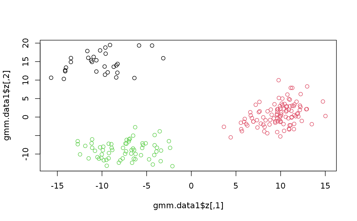
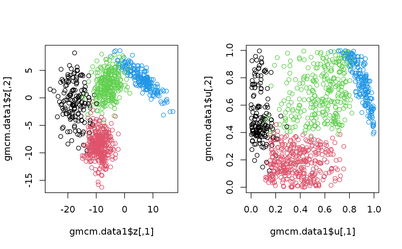
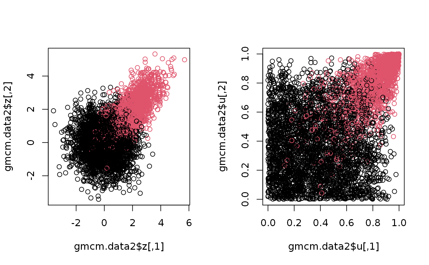
set.seed(2)

# Simulation from the GMM
gmm.data1 <- SimulateGMMData(n = 200, m = 3, d = 2)
str(gmm.data1)
#> List of 3
#>  $ z    : num [1:200, 1:2] 5.67 -5.11 -13.48 10.37 -9.9 ...
#>  $ K    : int [1:200] 2 3 1 2 3 3 1 3 3 3 ...
#>  $ theta:List of 5
#>   ..$ m    : num 3
#>   ..$ d    : num 2
#>   ..$ pie  : Named num [1:3] 0.127 0.481 0.393
#>   .. ..- attr(*, "names")= chr [1:3] "pie1" "pie2" "pie3"
#>   ..$ mu   :List of 3
#>   .. ..$ comp1: num [1:2] -9.62 15.85
#>   .. ..$ comp2: num [1:2] 9.68 1.26
#>   .. ..$ comp3: num [1:2] -7.1 -9.12
#>   ..$ sigma:List of 3
#>   .. ..$ comp1: num [1:2, 1:2] 7.6 1.13 1.13 6.84
#>   .. ..$ comp2: num [1:2, 1:2] 3.53 1.79 1.79 8.33
#>   .. ..$ comp3: num [1:2, 1:2] 7.73 1.37 1.37 4.81
#>   ..- attr(*, "class")= chr "theta"

# Plotting the simulated data
plot(gmm.data1$z, col = gmm.data1$K)

# Simulation from the GMCM
gmcm.data1 <- SimulateGMCMData(n = 1000, m = 4, d = 2)
str(gmcm.data1)
#> List of 4
#>  $ u    : num [1:1000, 1:2] 0.933 0.873 0.635 0.211 0.459 ...
#>  $ z    : num [1:1000, 1:2] 7.93 4.89 -5.2 -11.27 -7.68 ...
#>  $ K    : int [1:1000] 4 4 3 2 2 1 2 2 2 2 ...
#>  $ theta:List of 5
#>   ..$ m    : num 4
#>   ..$ d    : num 2
#>   ..$ pie  : Named num [1:4] 0.149 0.347 0.291 0.212
#>   .. ..- attr(*, "names")= chr [1:4] "pie1" "pie2" "pie3" "pie4"
#>   ..$ mu   :List of 4
#>   .. ..$ comp1: num [1:2] -17.24 -1.19
#>   .. ..$ comp2: num [1:2] -8.89 -8.69
#>   .. ..$ comp3: num [1:2] -5.58 2.39
#>   .. ..$ comp4: num [1:2] 5.94 3.49
#>   ..$ sigma:List of 4
#>   .. ..$ comp1: num [1:2, 1:2] 9.66 -2.56 -2.56 12.24
#>   .. ..$ comp2: num [1:2, 1:2] 5.967 0.188 0.188 4.982
#>   .. ..$ comp3: num [1:2, 1:2] 8.96 1.79 1.79 4.52
#>   .. ..$ comp4: num [1:2, 1:2] 16.96 -7.52 -7.52 4.25
#>   ..- attr(*, "class")= chr "theta"

# Plotthe 2nd simulation
par(mfrow = c(1,2))
plot(gmcm.data1$z, col = gmcm.data1$K)
plot(gmcm.data1$u, col = gmcm.data1$K)

# Simulation from the special case of GMCM
theta <- meta2full(c(0.7, 2, 1, 0.7), d = 3)
gmcm.data2 <- SimulateGMCMData(n = 5000, theta = theta)
str(gmcm.data2)
#> List of 4
#>  $ u    : num [1:5000, 1:3] 0.205 0.57 0.804 0.574 0.255 ...
#>  $ z    : num [1:5000, 1:3] -0.551 0.74 1.817 0.753 -0.357 ...
#>  $ K    : int [1:5000] 1 1 1 1 1 1 2 2 1 1 ...
#>  $ theta:List of 5
#>   ..$ m    : num 2
#>   ..$ d    : num 3
#>   ..$ pie  : Named num [1:2] 0.7 0.3
#>   .. ..- attr(*, "names")= chr [1:2] "pie1" "pie2"
#>   ..$ mu   :List of 2
#>   .. ..$ comp1: num [1:3] 0 0 0
#>   .. ..$ comp2: num [1:3] 2 2 2
#>   ..$ sigma:List of 2
#>   .. ..$ comp1: num [1:3, 1:3] 1 0 0 0 1 0 0 0 1
#>   .. ..$ comp2: num [1:3, 1:3] 1 0.7 0.7 0.7 1 0.7 0.7 0.7 1
#>   ..- attr(*, "class")= chr "theta"

# Plotting the 3rd simulation
par(mfrow=c(1,2))
plot(gmcm.data2$z, col = gmcm.data2$K)
plot(gmcm.data2$u, col = gmcm.data2$K)