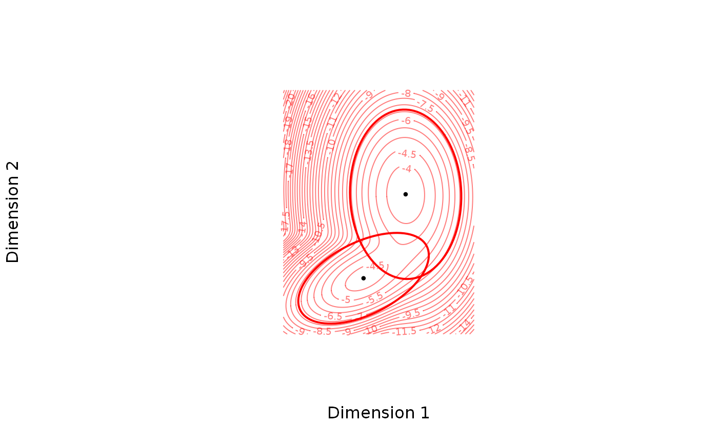
Visualizes the chosen dimensions of the theta object graphically by the GMM density and possibly the individual gaussian components.
# S3 method for theta
plot(x, which.dims = c(1L, 2L), n.sd = qnorm(0.99),
  add.means = TRUE, ..., add.ellipses = FALSE)
Arguments
| x | An object of class |
|---|---|
| which.dims | An integer vector of length 2 choosing which two dimensions to plot. |
| n.sd | An integer choosing the number of standard deviations in each dimension to determine the plotting window. |
| add.means | logical. If TRUE, dots corresponding to the means are added to the plot. |
| ... | Arguments passed to |
| add.ellipses | logical. If TRUE, ellipses outlining a 95% confidence
regions for each component are added in the bivariate multivariate
distribution defined by theta and |
Value
Plots via the contour function. Invisibly returns a list with
x, y, z coordinates that is passed to contour.
Author
Anders Ellern Bilgrau <anders.ellern.bilgrau@gmail.com>
Examples
set.seed(5)
theta <- rtheta(d = 3, m = 2)
if (FALSE) {
plot(theta)
plot(theta, col = "blue", asp = 1, add.means = FALSE)
plot(theta, col = "blue", asp = 1, add.means = TRUE)
plot(theta, which.dims = c(3L, 2L), asp = 1)
}
plot(theta, asp = 1, n.sd = 3, add.ellipses = TRUE,
     nlevels = 40, axes = FALSE,
     xlab = "Dimension 1", ylab = "Dimension 2")
